Blog #15: Worksheet 5.2- Cepheid Relations

Let's analyze real data about Cepheid Relations using Henrietta Swan Leavitt's actual date from 1908!

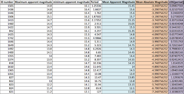
Included was a CSV file with the data.

(a) The data file, "Cepheid_variables.csv", contains data for 25 Cepheid variables located in the Small Magellanic Cloud (SMC). Each line contains a specific Cepheid's (1) ID number, (2) Maximum apparent magnitude, (3) Minimum apparent magnitude and (4) Period. Calculate the mean apparent magnitude for each Cepheid. 

In order to find the mean apparent magnitude, I simply took the minimum and maximum apparent magnitudes of each Cepheid and averaged the two.

Table 1: Cepheid Relations Chart

Since there were many individual Cepheids, I decided to get the mean apparent magnitude using Excel's "AVERAGE" function using the maximum and minimum apparent magnitudes as the input. The resulting mean apparent magnitude for each Cepheid is shown in the blue column in Table 1.


(b) The distance to the SMC is about 60 kpc, where kpc = 1000 pc. Convert your mean apparent magnitudes into mean absolute magnitudes. Plot the Cepheid mean absolute magnitudes as a function of period. This plot should look exponential. 

In order to get the mean absolute magnitude, I had to convert the mean apparent magnitude into the mean absolute magnitude using the equation:

\begin{align}
M = m - 5 \log {\left(\frac{d}{10 \text{ pc}}\right)}
\end{align}

where $m$ is the mean apparent magnitude, and $d$ is the distance to the SMC, which is 6000 pc. The values of this conversion for each Cepheid to its mean absolute magnitude are in Table 1 in the orange column.

The plot looks as follows:

Figure 1: Mean Absolute Magnitude vs. Period (days)

It does indeed look exponential.

(3) It is often handy to plot exponential (or power-law) functions with one or more logarithmic axes, which "straighten out" the data. Magnitudes are already exponential, so we don't need to adjust that axis. Plot the Cepheid mean absolute magnitudes as a function of $\log_{10}$(Period). Verify that the plot now looks linear. 

In order to plot the mean absolute magnitude against a linear axis, I converted the period of each Cepheid into the log of the period, as shown in the purple column in Table 1, and got the following chart:

Figure 2: Mean Absolute Magnitude vs. log(Period) in Days

(4) and (5)  Now that the data looks linear, we can estimate the parameters of the linear relation, $M_v(P) = A \log_{10}(\text{Period})+ B$. $A$ and $B$ are "free parameters" that allow the function to match the data. 

You can determine the precise values of A and B by minimizing the difference between the observed points and model using the metric:

\begin{align}
\chi^2 \equiv \sum_{i=1}^{25}(O_i - C_i)^2
\end{align}

where $O_i$ is the observed value and $C_i$ is the predicted (model) value.

In this case, $A = -2.0332$ and $B = -2.7276$.